for more information, contact Kenneth A. LaBel
![]()
J. Barth, NASA Goddard Space Flight Center
The definition of the radiation environment for SEE predictions must provide sufficient information to meet two criteria:
1) What is the "normal" radiation environment under which the system must operate? In other words, will the mitigation measures and mission operation plans be adequate to handle the SEU rates during normal operation times?
2) What is the "worst case" radiation environment that the mission will encounter? In other words, will the levels of radiation during a pass through the peak fluxes of the proton belts or at the peak of a solar flare result in catastrophic data loss or cause parts to experience permanent or semi-permanent damage?
This section is intended to inform SEECA users of the risks, unknowns, and uncertainties inherent in radiation environment predictions. Thus, they will be better able to define SEE mitigation requirements that reduce risk with reasonable cost.
The main sources of energetic particles that are of concern to spacecraft designers are:
1) protons and electrons trapped in the Van Allen belts,
2) heavy ions trapped in the magnetosphere,
3) cosmic ray protons and heavy ions, and
4) protons and heavy ions from solar flares.
The levels of all of these sources are affected by the activity of the sun. The solar cycle is divided into two activity phases: the solar minimum and the solar maximum. An average cycle lasts about eleven years with the length varying from nine to thirteen years [1, 2, 3]. Generally, the models of the radiation environment reflect the particle level changes with respect to the changes in solar activity.
From the information provided by the mapping of the trapped heavy ions by the SAMPEX satellite [4], we know that these ions do not have sufficient energy to penetrate the satellite and to generate the ionization in electronic parts necessary to cause SEEs. Also, electrons are not known to induce SEEs. Therefore, trapped heavy ions and trapped electrons are not included in a radiation environment definition for SEEs and will not be discussed in the sections below.
In the past, analyses of SEEs focused on energetic heavy ion induced phenomena. However, SEE data from recent spacecraft [5, 6, 7] have shown that newer, high density electronic parts can have higher upset rates from protons than from heavy ions because of their low threshold LET value. In addition, it is difficult to shield against the high energy protons that cause SEE problems within the weight budget of a spacecraft. As a result, any successful and cost effective SEE mitigation plan must include a careful definition of the trapped proton environment and its variations.
Protons are the most important component of the "inner" Van Allen belt. In the equatorial plane, the high energy protons (E>30 MeV) extend only to about 2.4 earth radii. The energies range from keV to hundreds of MeV. The intensities range from 1 proton/cm2/sec to 1 x 10⁵ protons/cm2/sec. The location of the peak flux intensities varies with particle energy. This is a fairly stable population but three known variations are important when defining requirements for SEE analyses. The most well known variation in the population is due to the cyclic activity of the sun. During solar maximum, the trapped proton populations near the atmospheric cut-off at the inner edge of the belt are at the lowest levels and, during solar minimum, they are at their highest. Second, the trapped protons are subject to perturbations at the outer edge of the inner belt and in the region between two and three earth radii due to geomagnetic storms and/or solar flare events. Last, the particle population is affected by the gradual change (secular variation) of the earth's magnetic field.
Trapped proton levels are calculated using the NASA AP8 model [8]. In the model, flux intensities are ordered according to field magnitude (B) and dipole shell parameter (L). The AP8 model comes in solar minimum and solar maximum versions, therefore, it is possible to take into account the solar cycle variations by simply selecting the appropriate model version. Otherwise, the models are static and do not reflect the variations due to storms and the geomagnetic field changes. Consequently, the trapped proton fluxes from the AP8 model represent omnidirectional, integral intensities that one would expect to accumulate on an average over a six month period of time. For limited durations, short term excursions for the models averages can reach orders of magnitude above or below.
Analyses of data gathered in flight before, during, and after geomagnetic storms and solar flare events have shown that the trapped proton population is affected by these phenomena at the outer edges of their trapping domain. It was observed on the CRRES satellite that flew during solar maximum that the so called "slot" region of the magnetosphere (2 < L < 3) can become filled with very energetic trapped protons as a result of solar flare events [9]. The decay time of the second belt is estimated to be on the order of 6-8 months. Phillips Laboratory has modeled this second proton belt as detected by the CRRES satellite [10]. The Air Force DMSP satellite flew during solar minimum. Particle flux monitors on board the DMSP showed that, after a major magnetic storm, the inner proton belt was reconfigured and eroded such that a second belt was formed [11]. A model of this redistribution of particles is not available.
To address the problem of the variation in the particle population due to the changes in the geomagnetic field, it has become a common practice to obtain fluxes from the AP8 model by using geomagnetic coordinates (B,L) calculated for the epoch of AP8 model (1964 for solar minimum and 1970 for solar maximum). This practice came about with the observation that, by using the actual epoch of the mission (e.g., 1995) for the geomagnetic coordinates for orbits at low altitudes (<1000 km), unrealistically high levels of fluxes are obtained from the models due to a lack of an atmospheric cutoff condition in the AP8 [12]. However, B,L coordinates calculated with 1964 and 1970 epochs must be used with caution because it has been shown by in-flight proton flux measurements at an altitude of 541 kilometers [13] that the predictions obtained with geomagnetic coefficients for 1970 can result in significant errors in the spatial placement of the particle populations. This error is usually averaged out when the proton fluence is orbit integrated over a period of 24 hours or greater but it can result in errors when specific positions in space are analyzed.
Galactic cosmic ray particles originate outside the solar system. They include ions of all elements from atomic number 1 through 92. The flux levels of these particles are low but, because they include highly energetic particles (10s of MeV/n ~ E ~ 100s of GeV/n) of heavy elements such as iron, they produce intense ionization as they pass through matter. As with the high energy trapped protons, they are difficult to shield against. Therefore, in spite of their low levels, they constitute a significant hazard to electronics in terms of SEEs.
As with the trapped proton population, the galactic cosmic ray particle population varies with the solar cycle. It is at its peak level during solar minimum and at its lowest level during solar maximum. The earth's magnetic field provides spacecraft with varying degrees of protection from the cosmic rays depending primarily on the inclination and secondarily on the altitude of the trajectory. However, cosmic rays have free access over the polar regions where field lines are open to interplanetary space. The exposure of a given orbit is determined by rigidity functions calculated with geomagnetic field models [14]. The coefficients in the models include a time variation so that the rigidity functions can be calculated for the epoch of a mission.
The levels of galactic cosmic ray particles also vary with the ionization state of the particle. Particles that have not passed through large amounts of interstellar matter are not fully stripped of their electrons. Therefore, when they reach the earth's magnetosphere, they are more penetrating than the ions that are fully ionized. The capacity of a particle to ionize material is measured in terms of LET and is primarily dependent on the density of the target material and to a lesser degree the density and thickness of the shielding material.
Several models of the cosmic ray environment are available including CREME [15], CHIME [16], and a model by Badhwar and O'Neill [17]. The model most commonly used at this time is CREME; however, CHIME is based on more recent data from the CRRES satellite. The authors of CREME recommend that most of the environment options available in CREME not be used because they are outdated or inaccurate [18]. They suggest that the standard solar minimum calculations be used for most applications (M=1) and that a worst case estimate should be obtained using the singly ionized model (M=4). Reference 16 compares the CHIME and CREME models and includes a brief discussion of the Badhwar and O'Neill model.
The CREME and CHIME models include solar cycle variations and magnetospheric attenuation calculations. The CREME model calculates LET for a simple shield geometry for aluminum shields and targets. CHIME improves the LET calculations by permitting the user to choose a shield material density and a target material density. Also, the CHIME model assumes that the anomalous component of the environment is singly ionized.
As mentioned in Section 3.1, work by Feynman et al. [2, 3] and Stassinopoulos et al. [1] shows that an average eleven year solar cycle can be divided into four inactive years with a small number of flare events (solar minimum) and seven active years with a large number of events (solar maximum). During the solar minimum phase, few significant solar flare events occur; therefore, only the seven active years of the solar cycle are usually considered for spacecraft mission evaluations. Large solar flare events may occur several times during each solar maximum phase. For example, in cycle 21 there were no events as large as the August 1972 event of cycle 20; whereas, there were at least eight such events in cycle 22 for proton energies greater than 30 MeV. The events last from several hours to a few days. The proton energies may reach a few hundred MeV and the heavy ion component ranges in energy from 10s of MeV/n to 100s of GeV/n. As with the galactic cosmic ray particles, the solar flare particles are attenuated by the earth's magnetosphere. The rigidity functions that are used to attenuate those particles can also be used to attenuate the solar flare protons and heavy ions. When setting part requirements, it is important to keep in mind that solar flare conditions exist for only about two percent of the total mission time during solar maximum.
An empirical model of the solar flare proton environment based on solar cycle 20 has existed since 1973 [19]. In 1974 King introduced a probabilistic model of the solar cycle 20 events [20]. This model divides events into "ordinary" and "anomalously large" (AL) and predicts the number of AL events for a given confidence level and mission duration. Stassinopoulos published the SOLPRO model [21] based on King's analysis. Since data for more solar cycles have become available, Feynman et al. [2, 3] have concluded that the proton fluence distributions actually form a continuum of events between "ordinary" the "anomalously large" flares. A team at JPL has combined the results of several works into the JPL Solar Energetic Particle Event Environment Model (JPL92) [22]. This model consists of three parts: a statistically based model of the proton flux and fluence, a statistically based model of the helium flux and fluence, and a heavy ion composition model.
The solar flare proton portion of the JPL92 model predicts essentially the same fluences as the SOLPRO code for the solar flare proton energies that are important for SEE analysis ( E>30 MeV). However, for worst case analyses, the peak solar flare proton flux is required and neither model contains this information. The peak flux of the protons for the August 1972 event can be obtained from the CREME model by specifying M=9 and element number = 1.
For the 26 events observed on the CRRES satellite [16], the peak fluxes for the helium ions with energies E > 40 MeV/n were three times higher than the galactic cosmic ray heavy ion levels. Above the energy of a few hundred MeV/n, the solar flare levels merge with those of the galactic cosmic ray background. The CREME model of the solar flares assumes that the solar particle events with the highest proton fluxes are always heavy ion rich. However, Reames et al. [23] contradict this assumption in their study of the ISEE 3 data. They found an inverse correlation between proton intensity and the iron/carbon heavy ion abundance ratio and that the composition of the flare was a result of the location of the flare on the sun.
The JPL92 model includes a definition of the solar flare heavy ion component based on the data from the IMP series of satellites. A paper by McKerracher et al. [24] gives an excellent overview of that model and presents sample calculations for interplanetary space at 1 AU. One of the findings of this work is that the JPL92 model calculates more realistic and lower solar heavy ion induced SEE rates. The CHIME model also contains a definition of the solar flare heavy ion fluence. As with the JPL92 model, it is expected that the CHIME model will predict lower SEE rates due to solar heavy ions.
There are extremely large variations in the SEE inducing flux levels that a given spacecraft encounters depending on its trajectory through the radiation sources. Some of the typical orbit configurations are discussed below with emphasis given to considerations that are important when calculating SEE rate predictions.
The most important characteristic of the environment encountered by satellites in LEOs is that several times each day they pass through the proton and electron particles trapped in the Van Allen belts. The level of fluxes seen during these passes varies greatly with orbit inclination and altitude. The greatest inclination dependencies occur in the range of 0°< i < 30°. For inclinations over 30°, the fluxes rise more gradually until about 60°. Over 60° the inclination has little effect on the flux levels. The largest altitude variations occur between 200 to 600 km where large increases in flux levels are seen as the altitude rises. For altitudes over 600 km, the flux increase with increasing altitude is more gradual. The location of the peak fluxes depends on the energy of the particle. For trapped protons with E > 10 MeV, the peak is at about 4000 km. For normal geomagnetic and solar activity conditions, these proton flux levels drop gradually at altitudes above 4000 km. However, as discussed above, inflated proton levels for energies E > 10 MeV have been detected at these higher altitudes after large geomagnetic storms and solar flare events.
The amount of protection that the geomagnetic field provides a satellite from the cosmic ray and solar flare particles is also dependent on the inclination and to a smaller degree the altitude of the orbit. As altitude increases, the exposure to cosmic ray and solar flare particles gradually increases. However, the effect that the inclination has on the exposure to these particles is much more important. As the inclination increases, the satellite spends more and more of its time in regions accessible to these particles. As the inclination reaches polar regions, it is outside the closed geomagnetic field lines and is fully exposed to cosmic ray and solar flare particles for a significant portion of the orbit.
Under normal magnetic conditions, satellites with inclinations below 45° will be completely shielded from solar flare protons. During large solar events, the pressure on the magnetosphere will cause the magnetic field lines to be compressed resulting in solar flare and cosmic ray particles reaching previously unattainable altitudes and inclinations. The same can be true for cosmic ray particles during large magnetic storms.
Highly elliptical orbits are similar to LEO orbits in that they pass through the Van Allen belts each day. However, because of their high apogee altitude (greater than about 30,000 km), they also have long exposures to the cosmic ray and solar flare environments regardless of their inclination. The levels of trapped proton fluxes that HEOs encounter depend on the perigee position of the orbit including altitude, latitude, and longitude. If this position drifts during the course of the mission, the degree of drift must be taken into account when predicting proton flux levels.
At geostationary altitudes, the only trapped protons that are present are below energy levels necessary to initiate the nuclear events in materials surrounding the sensitive region of the device that cause SEEs. However, GEOs are almost fully exposed to the galactic cosmic ray and solar flare particles. Protons below about 40-50 MeV are normally geomagnetically attenuated, however, this attenuation breaks down during solar flare events and geomagnetic storms. Field lines that cross the equator at about 7 earth radii during normal conditions can be compressed down to about 4 earth radii during these events. As a result, particles that were previously deflected have access to much lower latitudes and altitudes.
The evaluation of the radiation environment for these missions can be extremely complex depending on the number of times the trajectory passes through the earth's radiation belts, how close the spacecraft passes to the sun, and how well known the radiation environment of the planet is. Each of these factors must be taken very carefully into account for the exact mission trajectory.
Careful analysis is especially important for missions that fly during solar maximum and that have trajectories that place the spacecraft close to the sun. Guidelines for scaling the intensities of particles of solar origin for spacecraft outside of 1 AU have been determined by a panel of experts [25]. They recommend that a factor of 1 AU x 1/r2 be used for distances less than 1 AU and that values of 1 AU x 1/r3 be used for distances greater than 1 AU.
| Radiation Source | Models | Effects of Solar Cycle | Variations | Types of Orbits Affected |
|---|---|---|---|---|
| Trapped Protons | AP8-MIN; AP8-MAX | Solar Min - Higher; Solar Max - Lower | Geomagnetic Field; Solar Flares; Geomagnetic Storms | LEO; HEO; Transfer Orbits |
| Galactic Cosmic Ray Ions | CREME; CHIME; Badhwar & O'Neill | Solar Min - Higher; Solar Max - Lower | Ionization Level | LEO; GEO; HEO; Interplanetary |
| Solar Flare Protons | SOLPRO; JPL92 | Large Numbers During Solar Max; Few During Solar Min | Distance from Sun Outside 1 AU; Orbit Attenuation; Location of Flare on Sun | LEO (I>45°); GEO; HEO; Interplanetary |
| Solar Flare Heavy Ions | CREME; JPL92; CHIME | Large Numbers During Solar Max; Few During Solar Min | Distance from Sun Outside 1 AU; Orbit Attenuation; Location of Flare on Sun | LEO; GEO; HEO; Interplanetary |
Actual flight data have shown that SEE rates are clearly influenced by the dynamics of the radiation environment. The section above mentions some of the uncertainties inherent in predicting the radiation environment for a mission. The purpose of this section is to specifically address the factors that must be considered to reduce uncertainties.
Experience has shown that the most effective means of reducing uncertainty factors and design margins in particle predictions is to define for the mission:
1. when the mission will fly,
2. where the mission will fly
,
3. mission duration,
4. when the systems will be deployed,
5. what systems must operate during worst case environment conditions,
6. what systems are critical to mission success, and
7. the amount of shielding surrounding the SEE sensitive part(s).
We caution against using old predictions from previous missions. As discussed in the sections above, the predictions have large variations that are a function of altitude, inclination, model used, and time of the mission.
Particle level predictions based on the actual mission scenarios are lower than those based on taking the worst case prediction for every environment. Estimates that include only worst case conditions lead to over-design and should be used only in the concept design phase of a mission when the actual launch date and length have not been defined. After the launch date and duration are defined, it is possible to estimate how long the spacecraft will be in each phase of the solar cycle. These estimates should consider the impact of a launch delay of one year. Mission scenario definition is especially important for solar flare particles where the number of events is highly dependent on the amount of time that the satellite spends in solar maximum conditions.
The uncertainty factor defined for the trapped proton AP8 model is two. This is based on the statistical error inherent in merging the several spacecraft data sets that make up the model and does not include the substantial variations that occur over time. The largest variability in the trapped proton predictions is a function of the trajectory of the spacecraft. Therefore, applying proton predictions for a satellite in one orbit trajectory to another trajectory can result in errors up to several orders of magnitude.
To reduce the uncertainty of trapped proton calculations for SEE application, the definition of the trapped proton environment must specifically take into account:
1. how long the mission will be in each phase of the solar cycle and the effect of
changes in the launch date,
2. the orbit trajectory,
3. analysis of the effects of the secular variation of the geomagnetic field
(especially for orbits under 1000 km),
4. analysis of the variation in the outer edges of the proton trapping regions due
to solar flare events/magnetic storms, and
5. the amount of spacecraft shielding surrounding the SEE sensitive part(s).
The basic uncertainty factor defined for the CREME model is two. The CHIME model will provide more updated abundances when it is available.
To reduce the uncertainty in the predictions of the galactic cosmic ray heavy ion levels, the definition must consider:
1. how long the mission will be in each phase of the solar cycle and the effect
of changes in the launch date,
2. the effect of the ionization state of the anomalous component,
3. the amount of geomagnetic shielding for the orbit, and
4. estimate of the amount of shielding surrounding the SEE sensitive part(s).
The component of the environment that presents the largest uncertainty in predictions is the solar flare protons. Some solar cycles (Cycle 21) contain no extremely large flares at all. Other cycles contain as many as eight extremely large events (Cycle 22). The problem of providing solar flare predictions to those concerned with SEE criticality analysis is compounded by the limitations of the models. They are designed for determining mission integrated total dose or solar cell degradation levels and do not adequately address the SEE problem. That is, they provide event integrated fluences (SOLPRO) or mission integrated and daily fluences (JPL92). These values are not adequate for determining worst case SEE vulnerability during the peak flux levels of the flares. The new CHIME model promises to provide these options for users when it becomes available. In the meantime, the best option is to use the peak flux spectrum from the August 1972 event [14]. The fluence levels provided by the SOLPRO and JPL92 models are a function of confidence level and mission duration.
To reduce the uncertainty in solar flare proton predictions, the definition must take into account:
1. how long the mission will be in each phase of the solar cycle and the effect
of changes in the launch date,
2. the level of confidence selected by the project,
3. fluence levels for an extremely large event,
4. flux levels for the peak of an event,
5. the amount of geomagnetic shielding for the orbit,
6. estimate of how many times such an event will occur, and
7. the amount of shielding surrounding the SEE sensitive part(s).
The JPL92 model provides a significant improvement over the CREME model for the solar flare heavy ion compositions. As with the solar flare proton portion of the model, the heavy ion model gives fluences as a function of confidence level and mission duration. Again, for SEE analysis, a peak spectrum must be analyzed for worst case conditions.
The solar flare heavy ion predictions must take into account:
1. how long the mission will be in each phase of the solar cycle and the effect
of changes in the launch date,
2. the level of confidence selected by the project,
3. fluence levels for an extremely large event,
4. flux levels for the peak of an event,
5. the amount of geomagnetic shielding for the orbit,
6. estimate of how many times such an event will occur, and
7. the amount of shielding surrounding the SEE sensitive part(s).
It is not as easy to define the radiation environment for SEE requirements as for TID requirements. In specifying a TID environment, all components of the environment (electrons, protons, bremsstrahlung) are converted to dose units (rads) and summed. The SEE-inducing environment may consist of both protons and heavy ions. Since the underlying physics of the interactions of protons and heavy ions are different, the SEE prediction models and the environment input required are not the same. In general, heavy ions cause upsets via direct ionization of the sensitive regions in the device. The LET spectrum for the particular orbit is used to define this portion of the SEE-inducing radiation environment. Proton-induced upsets are usually caused by secondaries produced by nuclear collisions in the material surrounding the sensitive node of the device. The energy of the incident proton is the best predictor of the damage potential as it determines the levels of secondary heavy ions produced by the collisions. Therefore, the proton energy spectrum is used to define this component of the SEE-inducing radiation environment. In rare cases, where the LET threshold of the device is very low (< 1 MeV*cm2/mg), the protons can directly ionize the sensitive regions. One example is the 1773 fiber optic data bus. In these situations, the LET spectrum of the protons is used, rather than the proton energy spectrum.
SEE predictions are further complicated by the large variation in the criticality levels of system components. For example, it is not necessary to apply worst case solar flare proton conditions that occur for only a few days of the mission to a data recording system that is not required to maintain data integrity during the flares. These are "normal operation" conditions, hence, environments to consider are daily averages, worst case passes through the South Atlantic Anomaly (SAA), and background cosmic ray heavy ions. On the other hand, devices that control critical functions must be able to operate at all times and may have the requirement that no SEEs are permitted. If this is the case, worst case environments are defined and applied, such as, peak fluxes in the SAA and peak solar flare conditions.
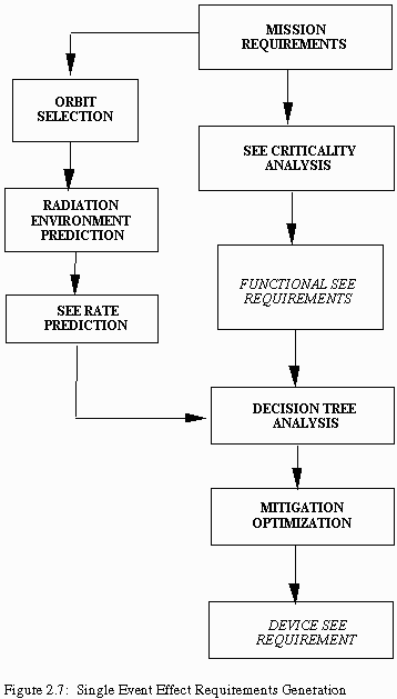
It is most advantageous to a mission if the radiation environment specialist is involved as soon as mission requirements are set. In fact, there are cases where it benefits the mission to have advice on radiation environment levels during the orbit selection process. Experience has shown that it is possible to reduce radiation exposure by choosing more benign regions of space while still meeting mission goals. In the SEE requirements generation flow (Figure 2.7), the radiation environment prediction and subsequent SEE predictions for the parts on the preliminary parts list occurs in parallel with setting system functional requirements. At this phase in the mission, a nominal shielding value must be set (e.g., 60 mils). The environment predictions and SEE predictions will be for this shielding value in the requirements generation at the point where decision tree analysis begins.
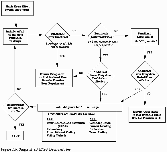
After setting functional requirements and predicting SEE rates, device sensitivity and criticality are taken into account if further mitigation is necessary. (See Figure 2.6, Single Event Decision Tree). In the case of devices with a low threshold LET (implying probable sensitivity to protons), it may be beneficial to evaluate the actual shielding geometry to determine if a lower, more accurate SEE prediction can be defined. The obvious advantage of this "mitigation" approach is the potential cost savings in eliminating or reducing design impacts. In the case of heavy ions, shielding is not likely to have an effect on the rate of SEE occurrence.
After mission planners have determined the mission specifications, they should provide the radiation environment specialists with:
1. the orbit configuration,
2. the date of launch,
3. the mission duration, and
4. the nominal shielding thickness(es).
The definition of the radiation environment for SEE analyses based on the above parameters should include (if applicable for the orbit):
1. trapped proton spectra attenuated by the nominal shielding thickness(es) for:
a. orbit averaged daily fluences,
b. fluences for worst case pass through the SAA, and
c. peak fluxes in the SAA;
2. LET spectrum for the nominal shield thickness(es) for orbit attenuated, galactic cosmic ray heavy ions;
3. orbit attenuated solar flare proton spectra attenuated by the nominal shielding
thickness(es) for:
a. an entire solar flare event and
b. the peak of an event;
4. LET spectrum for the nominal shield thickness(es) for orbit attenuated, solar
heavy ions for:
a. an entire solar flare event and
b. an the peak of an event.
If any devices are susceptible to direct ionization by protons, it is necessary to include the LET spectrum for trapped and solar flare protons for the nominal shielding thickness(es) in the definition of the radiation environment.
![]()
1. E.G. Stassinopoulos, G.J. Brucker, D.W. Nakamura, C.A. Stauffer, G.B. Gee, J.L. Barth, "Solar Flare Proton Evaluation at Geostationary Orbits for Engineering Applications," accepted for publication in IEEE Special Transactions of Nuclear Science, April 1996.
2. J. Feynman, T.P. Armstrong, L. Dao-Gibner, and S. Silverman, "New Interplanetary Proton Fluence Model," J. Spacecraft, Vol. 27, No. 4, pp. 403-410, Jul.-Aug. 1990.
3. J. Feynman and S. Gabriel, "A New Model for Calculation and Prediction of Solar Flare Proton Fluences," AIAA 90-0292, 28th Aerospace Sciences Meeting, Reno, Nevada, Jan.8-11, 1990.
4. J.R. Cummings, A.C. Cummings, R.A. Mewaldt, R.S. Selesnick, E.C. Stone, T.T. von Rosenvinge, and J.B. Blake, "SAMPEX Measurements of Heavy Ions Trapped in the Magnetosphere," IEEE Trans. on Nuc. Sci., Vol. 40, No. 6, pp. 1458-1462.
5. K.A. LaBel, S. Way, E.G. Stassinopoulos, C.M. Crabtree, J. Hengemihle, and M.M. Gates, "Solid-state Tape Recorders: Spaceflight SEU Data for SAMPEX and TOMS/Meteor-3," IEEE Radiation Effects Data Workshop Record, pp. 77-84, 1993.
6. A. Campbell, P. McDonald, and K. Ray, "Single Event Upset Rates in Space," IEEE Trans. on Nuc. Sci., Vol. 39, No. 6, pp. 1829-1835, December 1992.
7. J. Adolphsen, J.L. Barth, E.G. Stassinopoulos, T. Gruner, M. Wennersten, K.A. LaBel, C.M. Seidleck, "Single Event Upset Rates on 1 Mbit and 256 Kbit Memories: CRUX Experiment on APEX," IEEE Trans. on Nuc. Sci., Vol. 42, No. 6, pp. 1964-1974, December 1995.
8. D.M. Sawyer and J.I. Vette, "AP-8 Trapped Proton Environment for Solar Maximum and Solar Minimum," NSSDC/WDC-A-R&S, 76-06, December 1976.
9. E.G. Mullen, M. S. Gussenhoven, K. Ray, and M. Violet, "A Double-peaked Inner Radiation Belt: Cause and Effect as Seen on CRRES," IEEE Trans. on Nuc. Sci., Vol. 38, No. 6, pp. 1713-1717, December 1991.
10. M.S. Gussenhoven, E.G. Mullen, M.D. Violet, C. Hein, J. Bass, and D. Madden, "CRRES High Energy Proton Flux Maps," IEEE Trans. on Nuc. Sci., Vol 40, No. 6, pp. 1450-1457, December 1993.
11. M.S. Gussenhoven, E.G. Mullen, and E. Holman, "Radiation Belt Dynamics During Solar Minimum," IEEE Trans. on Nuc, Sci., Vol. 36, No. 6, pp. 2008-2014, December 1989.
12. P.D. McCormick, "Radiation Dose and Shielding for the Space Station," Acta Astronautica, 17, p. 231, 1988.
13. C.S. Dyer, A.J. Sims, P.R. Truscott, J. Farren, and C. Underwood, "Radiation Environments on Shuttle Missions Using the CREAM Experiment," IEEE Trans. on Nuc. Sci., Vol. 39, No. 6, pp. 1809-1816, December 1992.
14. IAGA Working Group, "International Geomagnetic Reference Field, 1991 Revision", EOS Transactions of AGU, Vol. 73, No. 16, April 21, 1992.
15. J.H. Adams, Jr., "Cosmic Ray Effects on Microelectronics, Part IV," NRL Memorandum Report 5901, December 31, 1987.
16. D.L. Chennete, J. Chen, E. Clayton, T.G. Guzik, J.P. Wefel, M. Garcia-Munoz, C. Lapote, K.P. Ray, E.G. Mullen, and D.A. Hardy, "The CRRES/SPACERAD Heavy Ion Model of the Environment (CHIME) for Cosmic Rays and Solar Particle Effects on Electronic and Biological Systems in Space," Trans. on Nuc. Sci., Vol. 41, No. 6, pp. 2332-2339, December 1994.
17. G.D. Badhwar and P.M. O'Neill, "An Improved Model of the Galactic Cosmic Radiation for Space Exploration Missions," Nucl. Tracks Radiat. Meas., 20, No. 3, pp. 403-410, 1992.
18. E.L. Petersen, J.C. Pickel, J. H. Adams, Jr., and E.C. Smith, "Rate Prediction for Single Event Effects - A Critique," IEEE Trans. on Nuc. Sci., Vol. 39, No. 6, pp. 1577-1599, December 1992.
19. E.G. Stassinopoulos and J.H. King, "Empirical Solar Proton Model for Orbiting Spacecraft Applications," IEEE Trans. on Aerospace and Electronic Systems, Vol. AES-10, No. 4, pp. 442-450, July 1974.
20. J.H. King, "Solar Flare Proton Fluences for 1977-1983 Space Missions," J. Spacecraft and Rockets," 11: pp. 401-408, 1974.
21. E. G. Stassinopoulos, "SOLPRO: A Computer Code to Calculate Probabilistic Energetic Solar Flare Fluences," NSSDC 75-11, National Space Science Data Center, Greenbelt, Maryland, April 1975.
22. G. Murphey, D. Croley, M. Cherng, and G. Spitale, "The JPL Solar Energetic Particle Event Environment Model," presentation material from September 1992.
23. D. V. Reames, H. V. Cane, and T. T. von Rosenvinge, "Energetic Particle Abundances in Solar Electron Events," The Astrophys. J., 357, pp. 259-270, July 1, 1990.
24. P. L. McKerracher, J. D. Kinnison, and R. H. Maurer, "Applying New Solar Flare Particle Event Models to Interplanetary Satellite Programs," IEEE Trans. on Nuc. Sci., Vol. 41, No. 6, pp. 2368-2375, December 1994.
25. M.A.Shea et al., "Toward a Descriptive Model of Solar Particles in the Heliosphere", Workshop on Interplanetary Charged Particle Environment, JPL, March 1987.
![]()
Introduction
1. The SEE Problem
2. Functional Analysis and Criticality
3. Ionizing Radiation Environment Concerns
4. Effects in Electronic Devices and SEE Rates
5. SEU Propagation Analysis: System Level Effects
6. SEE Mitigation: Methods of Reducing SEE Impacts
7. Managing SEEs: System Level Planning
8. SEE Criticality Assessment Case Studies
![]()